Cohomolgy-Some Module theory

 Preliminaries:
Given two modules $B,C$ we seek a module $A$ such that $B$ contains an isomorphic copy of $A$ such that resulting quotient module $B/A$ is isomorphic to $C$.
Clearly, $B$ contains an isomorphic copy of $A$ is same as saying that there is an injective homomorphism $\psi:A \rightarrow B$. This can be expressed as
$$A\equiv \psi (A)\subset B$$
To say $C$ is isomorphic to quotient means that there is a surjective homomorphism $\phi: B\rightarrow C$ with $ker\;\phi=\psi(A)$.
This gives us a pair of homomorphisms
$$A\stackrel{\psi }{\to }B\stackrel{\varphi }{\to }C$$
such that $im\;\psi=ker\;\phi$.

These homorphisms such that above holds are known as "exact".

Examples:

Using direct sum of modules $A,C$ with $B=A \oplus C$, the following exact sequence can be constructed.
$$0\to A\stackrel{i}{\to }A\oplus C\stackrel{\pi }{\to }C\to 0$$
where $i(a)=(a,0)$ and $\pi(a,c) = c$. Notice that $pi \circ i=\pi(a,c)\circ(a,0)=\pi(a,0)=0$. Thus $\partial^2=0$ map is satisfied.

When $A=Z$ a $Z$ module with $C=Z/nZ$, above sequence becomes
$$\begin{array}{r}0\to Z\stackrel{i}{\to }Z\oplus Z/nZ\stackrel{\pi }{\to }Z/nZ\to 0\\ 0\to Z\stackrel{n}{\to }Z\stackrel{\pi }{\to }Z/nZ\to 0\end{array}$$
If we consider $A=Z$ and $C=Z/nZ$, we can consider these as extension of $C$ by $A$.

For homomorphism $\phi$, we may form the following.
$$0\to K\stackrel{i}{\to }F(S)\stackrel{\varphi }{\to }M\to 0$$
Here $\phi$ is a unique $R$-module homomorphism which is identity in $S$ - set of generators for $M$ an $R$-module.k

K-Algebras and Bimodules

K-algebras

A k-algebra A is a (possibly noncommutative) ring with identity that is also a k-vector space, such that for α ∈ k and a,b ∈ A,

(1.1) α(ab) = (αa)b = a(αb).

Note that scalar commutes with ring elements.

Examples:

• Field extensions such as $F/E$.
• Polynomial ring $k[X,Y,Z]$.
• Matrix $M_{nm}(k)$ ring (under addition and multiplication) is $k$ algebra. Here we can see that $k$ can commute with elements of $M_{nm}(k)$ but the ring multiplication is non-commutative.
• The set $Hom_k(V,V)$ of $k$-linear maps of $k$ vector spaces forms a $k$-algebra under addition and composition of linear maps.
  

Since center of ${\cal H}$ consists of real numbers, ${\cal H}$ is a ${\cal R}$ algebra.

Finite dimensional $k$ algebra it is a finite dimensional vector space over $k$.

Note ${\cal C}$ is 2 dimensional over ${\cal R}$ etc.,

Bimodules

If $R,S$ are two rings, an $R-S$ bimodule is an abelian group $(M,+)$ such that

• $M$ is a left $R$ module, and a right $S$ module.
• for all $r \in R$, $s \in S$ and $m \in M$ \begin{equation}
  \label{eq:rs}
  (rm)s=r(ms)
  \end{equation}
  

An $R-R$ bimodule is known as $R-$bimodule.

For positive intergers $m,n$, the set of $n \times m$ matrices $M_{nm}(\mathcal{R})$. Here the $R$-module is $n \times n$ matrices $M_{nn}(\mathcal{R})$. And the $S$-module is $m \times m$ matrices $M_{mm}(\mathcal{R})$.

Addition and multiplication are carried out using the usual rules of matrix addition and matrix multiplication; the heights and widths of the matrices have been chosen so that multiplication is defined.

The crucial bimodule property, that $(rx)s = r(xs)$, is the statement that multiplication of matrices is associative.

A ring $R$ is a $R-R$ module.

For $M$ an $S-R$ bimodule and $N$ a $R-T$ bimodule then $M \otimes N$ is a $S-T$bimodule.

Bimodule homomorphism:

For $M,N$ $R-S$ bimodule, bimodule homomorphism $f:M \rightarrow N$ is an right $R$ module homomorphism as well as an right $S$ modules homomorphism.

An $R-S$ bimodule is same as left module over ring $R \otimes_Z S^{op}$ where $S^{op}$ is opposite ring of $S$. Note in opposite ring multiplication is performed in opposite direction of the original ring.

This caused me some confusion initially. $S^{op}$ is a ring with multiplication reversed. Denote multiplication in the righ $S$ by "." and opposite multiplication by "*". So, how does all this work to define a bimodule?
Lets look at $R \otimes_Z S^{op}$ operating on $m \in M$.
$$rs\ast m=rm.s=(rm)s=r(ms)$$
Thus the definition is satisfied. Using $R \otimes_Z S^{op}$ is more nicer.

Associative algebras-some preliminary notes

Associative algebra:

Associative algebras are generalizations of field extensions and matrix algebras. For example, in field extension $E/F$,$E$ can be considered a $F$-algebra of dimension $n$. Also a $F$-vector space.

An associative algebra $\mathcal{A}$ is a ring, (with multiplication associative) with scalar multiplication and addition from a field $F$.

$K$-algebra means an associative algebra over field $K$.

In short, we want the $F$ action to be compatible with multiplication in $\mathcal{A}$. Say $f \in F$ and $a,b \in \mathcal{A}$ then
$$(f.a)b=f.(ab)=a(f.b)$$

We may consider $F$ as a subring under identification $f \rightarrow f.1_A$ where $1_A$ is multiplicative identity. Then, in compatibility condition noted above we can drop the dot in between $F$ elements and $\mathcal{A}$ elements
$$fab=afb$$
which is same as saying $fc=cf$ for some $c=ab$. Hence, this implies that $F \in Z(\mathcal{A})$ - that is in center of $\mathcal{A}$.



Examples:
A standard first example of a $K$-algebra is a ring of square matrices over a field $K$, with the usual matrix multiplication.

Let $F=Q$, the field of rationals. Consider the polynomial $X^2-2 \in Q[X]$. The splitting field $E=Q(\sqrt{2})$. Then $Q(\sqrt{2})=\{a+b\sqrt{2}|a,b\} \in Q$ is a vector space of $F$ over $E$ such that $dim_F(E)=2$.

Note, that an $n$-dimensional $F$-algebra $A$ can be realized as a subalgebra of $M_n(F)$ ($n\times n$ matrices over field $F$).

If $A,B$ are $F$-algebras, they can be added and multiplied via tensor operations. That is $A \otimes_F B$ and $A \oplus B$ are also associative algebras.

If $A$ is an algebra of dimension $2$, then $A \equiv F \oplus F$. This means $A$ is quadratic extension of $F$, or $A$ contains a nilpotent element.

To prove this, first we establish commutativity of $A$ using basis $\{1,\alpha\}$ over $F$.
 To see this simply expand $(x+y\alpha)(x'+y\alpha')$
 
 Quadratic extension requires that every non-zero element of $A$ should be invertible.

 Say $x+y\alpha$ be a non-zero element that is not invertible. This means $y \neq 0$ and can assert $\alpha$ is not invertible.

 $A$ can be represented via subalgebra of $M_2(F)$. So, we write $\alpha$ as
 $$\begin{array}{r}\alpha =[[a,b],[c,d]]\text{ a 2 by 2 matrix }\end{array}$$
 Using above it is not too difficult to prove that $A \equiv F \oplus F$.

 Opposite algebras $A^{opp}$ is an algebra where multiplication is in reverse order. That is for $a,b \in A$, with $a.b$ as multiplication in $A$ and using $\times$ symbol for multiplication in $A^{opp}$, the condition is $b \times a = a.b$.
 

Cohomology-Homotopy operator etc.,

Homotopy equivalent manifolds have isomorphic de Rahm cohomology groups.

Suppose $F,G:M\rightarrow N$ are smooth homotopic maps. Suppose $\omega$ is a $k$ form on $N$ and $h$ be an homotopic operator that maps from space of $k$ forms on $N$ to $k-1$ forms on $M$ given by
$$d(h\omega )+h(d\omega )=G^{\ast }(\omega )-F^{\ast }(\omega )$$
This means $h:\mathcal{A}^k(N) \rightarrow \mathcal{A}^{k-1}(M)$.

This homotopy is used as a stepping stone for proving homotopy equivalent manifolds have isomorphic homology groups.

I shall write in detail the motivation and how this is used later.

There is deRahm theorem proof of which I shall blog later.

Cohomology- Homotopy

Imagine you are stuck in a strange planet without light source and it is always dark. You landed in an area with some rocks and some pleasant flat ground (otherwise, how else could you have landed?). Your job is to direct an incoming ship to a flat ground.

Since you took some algebraic topology at college, you are a bonafide Mathematician and would always think as one. So using your knowledge, you design this highly contrived, non-optimal "rock" detection system. (If you need more convincing Mathematician's way of doing certain simple things is unique, please refer to Mathematician's way of making Tea- Check out fantastic online book http://www.topologywithouttears.net).

Your plan or device has the following steps.
1. Put a peg on the ground at a random place. Tie a rope.
2. Walk in some direction for some time unrolling your rope, assuming that you haven't hit a rock, plant another peg where you tie other end of the rope.
3. Pause and recognize this rope as a curve on the surface and name it $f$.
4. Walk a few feet and repeat the same steps - if you are successful unrolling your rope, you have another curve - call is $g$.

Now if you can drag rope $f$ to rope $g$, you don't have a rock in between otherwise you have an obstruction or a rock!

If you can drag $f$ to $g$ (or vice versa), you call it $f ~ g$ and this basic idea of homotopy.

Now while dragging the rope from $f$ to $g$, you are working along a map $F$ which at start (we call the start as $t=0$ as a parameter for the drag), the map should be $f$ and at the end (say $t=1$) $F$ should be $g$.

This notion is formalized as follows. Let $M,N$ be two manifolds and let $f,g:M\rightarrow N$ be two smooth functions. If there is a $C^\infty$ map
$$F:M\times R\to N$$
such that $F(M,0) = f$ and $F(M,1)=g$, then we say $f$ is homotopic to $g$ and write $f \tilde g$.

Now that we have such a map, we can add extra nomenclature when certain conditions occur. Let $N=\mathcal{R}^n$. $F:M\times \mathcal{R} \rightarrow \mathcal{R}^n$ linear in $t$ can be expressed as
$$F(M,t)=f(1-t)+(t)g$$
When $t=0$ implies $F(M,0)=f$ and when $t=1$, $F(M,1)=g$.

Notice $F(M,t)=f+(g-f)t$ which is like $y=mx+c$ or a straight line equation in terms of $t$. Such a straight line path is called "Straight line homotopy".

Convex means that any arbitarary two points can be joined by a straight line.  On any subset of $\mathcal{R}^n$ for which this is true, straight line homotopy is applicable.

Sometimes we are fortune enough to get maps $f,g$ where $g:N \rightarrow M$ such that $f\circ g$ is identity on $N$ and $g \circ f$ is identity on $M$. In such situations, $M$ is considered to be "homotopy equivalent" to $N$. $M,N$ are said to be same homotopy type.

Notice, nothing precludes $N$ to be a single point set. For example, if $M=\mathcal{R}^n$ and $N$ is a single point set, we can smoothly scrunch $\mathcal{R}^n$ to a single point. Such manifolds that can be shrunk to a point are called "contractible".

Cohomology-Computations 1

Let $U,V$ be open cover of circle - $S^1$. Let $X,Y$ be arcs on the circle that correspond to the open cover with disjoint overlaps at top of the circle and at the bottom of the circle.

Each arc $X,Y$ is diffeomorphic to an interval and thus to $\mathcal{R}$.

Here instead of writing one forms and seeking existence of integral solutions, we can use Mayer-Vietoris sequence to make computations. The Mayer-Vietoris sequence for $S^1$ is as follows:
$$0\to H^0(M)\stackrel{i^{\ast }}{\to }{H}^0(U)\oplus H^0(V)\stackrel{j^{\ast }}{\to }{H}^0(U\cap V)\stackrel{d^{\ast }}{\to }{H}^1(M)\to 0.$$
Using dimensional formula for sequence of vector spaces $\sum_{k=0}^n(-1)^k d^k$, we can figure out dimension of $H^1(M)=d^1=1$ as follows:
$$1-2+2-d^1=0$$
Since $S^1$ is connected, $H^0(S^1)=\mathcal{R}$. As shown before $H^0(U)=H^0(V)=\mathcal{R}$. Since overlaps are disjoint we have $\mathcal{R} \oplus \mathcal{R}$. All this results in the following sequence.
$$0\to \mathcal{R}\stackrel{i^{\ast }}{\to }\mathcal{R}\oplus \mathcal{R}\stackrel{j^{\ast }}{\to }\mathcal{R}\oplus \mathcal{R}\to 0$$
Notice $j^*:H^{0}(U) \oplus H^{0}(V) \xrightarrow{j^*} H^{0}(U \cap V)$ is given as follows. Since, we are dealing with $0$ dimensional space, corresponding vectors are $0$ dimensionals - that is scalars or real numbers.
$$j^{\ast }(m,n)=(n-m,n-m)$$
That is these are elements of diagonal in $\mathcal{R}\times\mathcal{R}$. $d^*: H^{0}(U \cap V) \xrightarrow{d^*} H^{1}(M)$ sends this to one dimensional space which is isomorphic to $\mathcal{R}$, hence points $m \neq n$ will result in this element. Among many, we can choose one.

Cohomology-Mayers-Vietoris Long exact sequence.

The exact sequence of cochain complex
$$0\to {\mathrm{\Omega }}^{\ast }(M)\stackrel{i}{\to }{\mathrm{\Omega }}^{\ast }(U)\oplus {\mathrm{\Omega }}^{\ast }(V)\stackrel{j}{\to }{\mathrm{\Omega }}^{\ast }(U\cap V)\to 0$$
for some open cover $U,V$ of manifold $M$, yields a Long exact sequence in cohomology called 'Mayer-Vietoris' sequence.
$$\cdots H^{k-1}(U\cap V)\stackrel{d^{\ast }}{\to }{H}^k(M)\stackrel{i^{\ast }}{\to }{H}^k(U)\oplus H^k(v)\stackrel{j^{\ast }}{\to }{H}^k(U\cap V)\stackrel{d^{\ast }}{\to }{H}^{k+1}(M)\cdots$$
In this complex, $i^{*},j^{*}$ are induced from $i,j$. Since $H^k$ is quotient, the elements of $H^k$ are in cohomoloous classes. If we take a representative element $\sigma \in \Omega^{*}(M)$, then the map $i$ sends this element to $i\sigma$. Based on this, one can define $i^{*}$ as follows:
$$i^{\ast }([\sigma ])=([i\sigma ])=([i_U^{\ast }\sigma ],[i_V^{\ast }\sigma ])\in H^k(U)\oplus H^k(V)$$
Do similar thing to $j^{*}$, that is drop in equivalence classes instead of differential forms directly.
$$j^{\ast }([\omega ],[\tau ])=([j_V^{\ast }\tau -j_U^{\ast }\omega ])\in H^k(U\cap V)$$


To make all this work, we need a connecting homomorphism map $d^*$ defined as follows:
$$d^{\ast }[\eta ]=[\alpha ]\in H^{k+1}(M)$$
Since for $k \leq -1$, $\Omega^{k}(M)=0$, the sequence can be written as,
$$0\to H^0(M)\to H^0(U)\oplus H^0(v)\to H^0(U\cap V)\to H^0(M)\to \cdots$$


For a connected manifold, above sequence is exact.
$$0\to H^0(M)\to H^0(U)\oplus H^0(v)\to H^0(U\cap V)\to H^0(M)\to 0$$

Cohomology-Partition of Unity

Smooth manifolds are defined on nice topological spaces that have countable basis and are Hausdorff spaces. Partition of unity (POU) can be defined and existence proven more easily.

 Idea behind POU is as follows. Imagine a set of continuous functions defined on a topological space that takes values in the closed interval [0,1]. They are sort of functions that finitely many of them take non-zero values in a small neighborhood and vanish (become 0) in other places.

So how is all the above formalized? Given the niceness of topological space, we can defined these functions in the following manner.

1. Take an open cover $U_i$ of manifold $M$ such that at each point $x$ there
are finitely many open covers $U_i$.
2. Take a family of differential functions $0 \leq \beta_i(x)  \leq 1$ such that sum is unity at point x.
Such a family ${\beta_i(x)}$ define  on ${U_i}$ called  a POC subordinate to ${U_i}$.
3. These functions vanish beyond the ${U_i}$.
How's this useful?
On manifolds, integration of the forms can be done on a coordinate patch. POU helps extend this coordinate patch integration to whole manifold.
For an orientable manifold $M$, take a volume form $\omega$ at a point $p$.
$$\omega =h(p)d{x}^1\wedge d{x}^2\wedge \cdots d{x}^n$$
with postive definite $h(p)$ on a chart $U_i$ whose coordinate is $x=\phi(p)$.

Let $f:M \rightarrow R$ be a function on $M$. In the coordinate neighbourhood $U_i$ one can define integration of $n$-form as
$${\int }_{U_i}f={\int }_{{\varphi }_i(U_i)}f({\varphi }_i^{-1}(x))h({\varphi }_i^{-1}(x))d{x}^1\cdots d{x}^n$$
POU enables us to extend this integration over entire manifold.

Example: On $S^1$ , use open covers $U_1=S^1 - (1,0)$ and $U_2=S^1-(-1,0)$ to define "bump" functions
$\beta_1(\theta)=sin^2(\frac{\theta}{2})$ and $\beta_2(\theta)=cos^2(\frac{\theta}{2})$.
Since values of $sin$ and $cos$ belong to interval $[0,1]$ and sum of $\beta_1,\beta_2$ is always unity, it is easy to see that this a POU.

We can use this to integrate - say $\int_S^1 cos^2\theta$ over $S^1$.

$\beta_1(\theta)=sin^2(\frac{\theta}{2})$ and $\beta_2(\theta)=cos^2(\frac{\theta}{2})$.
This is a partition of Unity because,
1. $\beta_i(\theta) \in [0,1]$ for $i=1,2$.
2. if $p=(1,0)$ as $p \notin U_1$ results in value of function $0$. Similarly,
for $U_2$, at $p=(-1,0)$, value is $0$.
3. At any angle where both the functions are defined, POU acts as a weight that allocates a fraction to one function and rest of the fraction to next function. In our example, say we take $\theta = \pi/4$, $\beta_i(\pi/4)=1/2$, hence sum of $1/2+1/2=1$.

 We can use this to integrate - say $\int_{S^1} cos^2\theta$. Let us see what happens. Since POU acts as a weighting function that sums to $1$, we can allow overlaps in the integration. POU will allocate appropriate weight and make sure that the integration works as expected.
$${\int }_{s^1}co{s}^2(\theta )d\theta ={\int }_0^{2\pi }si{n}^2(\theta /2)co{s}^2(\theta )d\theta +{\int }_{-pi}^{pi}co{s}^2(\theta /2)co{s}^2(\theta )d\theta =\pi$$

Cohomology: Mayers-Vietoris sequence.

Let $U,V$ be an open cover of Manifold $M$. Remember it is very much possible that $U \cap V \neq \emptyset$.
Define the following inclusion maps
$$\begin{array}{r}{i}_u:U\to M,i_u(p)=p\\ i_v:V\to M,i_v(p)=p\\ j_U:U\cup V\to U,j_u(p)=p\\ j_V:U\cup V\to V,j_v(p)=p\end{array}$$
These inclusion map $i_U(p)=p$ from $U$ to $M$ and similar map $i_v(q)=q$ from $V$ to $M$ etc.,

Based on these inclusion maps one can define pull back maps of differentials
$$i_U^{\ast }:{\mathrm{\Omega }}^k(M)\to {\mathrm{\Omega }}^k(U)$$
Similarly one can define a pull back for $i_V$
$$i_V^{\ast }:{\mathrm{\Omega }}^k(M)\to {\mathrm{\Omega }}^k(V)$$
 Similar pull back maps are defined for $j_U,j_v$.
 $$\begin{array}{r}{j}_U^{\ast }:{\mathrm{\Omega }}^k(U\cup V)\to {\mathrm{\Omega }}^k(U)\\ j_V^{\ast }:{\mathrm{\Omega }}^k(U\cup V)\to {\mathrm{\Omega }}^k(V)\end{array}$$

 

 By restricting to $U$ and to $V$, we get a homorphism of vector spaces
 $$i:{\mathrm{\Omega }}^k(M)\to {\mathrm{\Omega }}^k(U)\oplus {\mathrm{\Omega }}^k(V)$$

 defined via
 $$\sigma \to (i_U^{\ast }\sigma ,i_V^{\ast }\sigma )$$

 Using this, define the difference map,
 $$j:{\mathrm{\Omega }}^k(U)\oplus {\mathrm{\Omega }}^k(V)\to {\mathrm{\Omega }}^k(U\cap V)$$
 by $j(\omega,\tau)=\tau-\omega$.

 This map indicates what to do with common vectors that belong to both $U$ and $V$. Similar maps are used in Finite dimensional vector spaces to prove dimensionality theorem when $U,V$ are subspaces whose intersection is non-empty.

 Here $\tau,\omega$ are pull backs maps shown before.
 $$\begin{array}{r}\omega =j_U^{\ast }\omega \\ \tau =j_v^{\ast }\tau \end{array}$$

 $j$ is a zero map when $U \cup V = \emptyset$.

 Proposition
 For each integer $k \geq 0$, the sequence
 $$0\to {\mathrm{\Omega }}^k(M)\stackrel{i}{\to }{\mathrm{\Omega }}^k(U)\oplus {\mathrm{\Omega }}^k(V)\stackrel{j}{\to }\mathrm{\Omega }(U\cap V)\to 0$$
 is exact.

 Proof:
 To show that this exact sequence, we need to show at each node image of previous function to this node is same as kernel from this node to next node.
 We will start with first node - $\Omega^k(M)$.
 $0$ vector maps every function to $0$ in the $\Omega^k(M)$ which is in kernel of $i$. Hence, $im\;(0\rightarrow \Omega^k(M))=ker\;i$.
 
 To prove exactness at $\Omega^k(U \cup V)$, we need to show that $j$ is surjective or onto as next maps takes everything to zero. Thus kernel of next map is all of $\Omega^k(U \cap V)$ which is range of $j$.
 
 We are already given $j$ map in the previous section. This map, together with a very nice partitions of unity, helps us to establish the onto of $j$ map.

 say $\omega \in \Omega^k(U \cap V)$. Let $p_U,p_v$ be functions that form partitions of unity. Define
$$\begin{array}{r}{p}_U\omega =\{\begin{array}{ll}{p}_v\omega \text{ when },& x\in U\cap V\\ 0\text{ otherwise },& x\in U-(U\cap V)\end{array}\\ p_V\omega =\{\begin{array}{ll}{p}_U\omega \text{ when },& x\in U\cap U\\ 0\text{ otherwise },& x\in V-(U\cap V)\end{array}\end{array}$$
The niceness of partition of unity allows the following to happen.
$$j(-p_u\omega ,p_v\omega )=p_v\omega +p_u\omega =\omega \text{ on }U\cap V$$
This shows that $j$ is onto and from the fact the next function sends everything to $0$, we have proved that this is a short exact sequence.

Cohomolgy-Long exact sequence

So far the following maps are defined.

• Cochain map $\phi:H^k(A)\rightarrow H^k(B)$ induced cohomology map
  $${\varphi }^{\ast }:H^k(A)\to H^k(B)$$
• For short exact sequence of cochain complexes $$0\to \mathcal{A}\stackrel{i}{\to }\mathcal{B}\stackrel{j}{\to }\mathcal{C}\to 0$$
  Connecting homomorphism map is
  $$d^{\ast }:H^k(\mathcal{C})\to H^{k+1}(\mathcal{A})$$
• Then the short exact sequence of cochain complexes
  $$0\to \mathcal{A}\stackrel{i}{\to }\mathcal{B}\stackrel{j}{\to }\mathcal{C}\to 0$$
  gives rise to long exact sequence in cohomology.
  $$\cdots H^{k-1}(\mathcal{C})\stackrel{d^{\ast }}{\to }{H}^k(\mathcal{A})\stackrel{i^{\ast }}{\to }{H}^k(\mathcal{B})\stackrel{j^{\ast }}{\to }{H}^k(\mathcal{C})\stackrel{d^{\ast }}{\to }{H}^{k+1}(\mathcal{A})\cdots$$
  
  

Cohomology-Connecting homomorphisms

A series of cochain complexes
$$0\to \mathcal{A}\to \mathcal{B}\to \mathcal{C}\to 0$$
is ``short exact'' if $i,j$ are cochain maps and for each $k$
$$0\to A\stackrel{i}{\to }B\stackrel{j}{\to }C\to 0$$
is short exact sequence of vector spaces.
Based on above sequence, we can define yet another new map called ``connecting homomorphism'' map

$d^{*}: H^k(\mathcal{C}) \rightarrow H^{k+1}(\mathcal{A})$

To analyze this connecting homomorphism,start with an element in $H^k(\mathcal{C})$ - say $c \in [c]$.
Since $C$ maps all elements to $0$ and because this is an exact sequence, image of $j$ will be onto. This means there exists an element $b\in B^k$ such that $c=j(b)$.
Because connecting homomorphism gives above commuting diagram, $C^{k+1}$ can be reached via $d(j(b))$ and also via $j(d(b))$. That is,
$$d(j(b))=j(d(b))$$
However, $c=j(b)$. Then, $d(j(b))=d(c)=0$. Thus the element $db (\in B^{k+1}) \in ker\;j$.

In the $k+1$ diagram $ker\;j=im\;i$. That means there is an element $db = i(a)$ for some $a \in A^{k+1}$. Since $i$ is injective, element $a$ is unique. Injectiveness of $i$ also means $i(da)=d(ia)=db=0$ which shows $a$ is co-cycle and defines a conjugacy class $[a]$.

The defining equation for connecting homomorphism is

$$d[c]=[a]\in H^{k+1}(A)$$

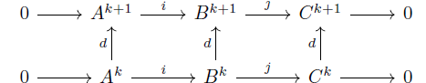
Cohomology of Cochain complex

Recall that the cochain $\mathcal{C}$ complex is not an exact sequence (condition $im\;d_{k-1}=\ker\:d_k$ won't hold). The following holds

$im\;d_{k-1} \subset ker\;d_k$.

This gives us an opportunity to define quotient space

$H^k(\mathcal{C})$ as $ker\;d_k / im\;d_{k-1}$ which measures cochain complex fails to be exact at $k$.

Terminology:

$ker\;d$ is k-cocyle or closed forms(DeRahm cohomology) and $im\;d$ is k-coboundary or exact forms (DeRahm cohomology). Elements of $H^k(\mathcal{C})$ are equivalent classes $[c]$ for $c \in ker\;d_k$ is called cohomology class.

cochain map:

Between any two cochain complexes $\mathcal{A}, \mathcal{B}$ one can define a cochain map $\phi:\mathcal{A} \rightarrow \mathcal{B}$ - a collection of linear maps $\phi_k:A_k \rightarrow B_k$. If $d_1,d_2$ are corresponding differential operators for $\mathcal{A},\mathcal{B}$, drawing a commuting diagram shows

$d_2\circ \phi_k = \phi_{k+1} \circ d_1$

Nice thing about this map is that induces map $\phi^{*}:H^k(\mathcal{A}) \rightarrow H^k(\mathcal{B})$ between cohomologies. This map is well defined because it takes exact forms to exact forms and closed forms to closed forms.

For $a \in Z^k(\mathcal{A})$ ie closed forms of $\mathcal{A}$ at $k$, $d(\phi(a))=\phi(d(a))=0$ and for $b \in \mathcal{A}^{k-1}$, easy to see that $\phi(d(b))=d(\phi(b))$.

Vector spaces-First isomorphism theorem

Let $T:V \rightarrow W$ be a linear transformation between vector spaces $V$ and $W$.

Then, $\tau:T/ker(W) \rightarrow Im(W)$ induces an isomorphism given by $\tau(v+ker(T)) = T(v)$.

First we need to establish that if $v+ket(T)$ is replaced by $v'+ker(T)$ for $v,v'$ in the same coset ie $v-v' \in ker(T)$, then  $T(v)=T(v')$. That is, we need to establish that above map is well defined.

Notice,

$T(v) = T( (v'-v)+v' ) = T(v-v')+T(v') = T(v')$

Then we need to establish that the map $\tau$ is a linear map.

That is, for $v,v' \in V$, we need to show that $\tau(v+ker(T) + v'+ker(T))=\tau(v+ker(T))+\tau(v'+ker(T))$.

Indeed,  $\tau(v+ker(T) + v'+ker(T)) = T(v+v'+ker(T)) =T(v)+T(v')=\tau(v+ker(T))+\tau(v'+ker(T)$.

And

$\tau(\alpha (v+ker(T))) = \tau(\alpha v + \alpha  ker(T) ) = T(\alpha v) = \alpha T(v) = \alpha \tau(v+ker(T))$.

Thus the map T/ker(W)$ is a linear map.

To prove isomorphism, we need to show that this map is one-one and onto.

For one-one, if $\tau(v+ker(T))=0$, need to show that $v+ker(T)=0$ which is a direct result of the observation that if $\tau(v+ker(T))=T(v)=0$, then $v \in ker(T)$.

For onto, just note any element of $im(T)$ can be written as $T(v)$ for some $v \in V$ and thus equal to $\tau(v+im(T))$.

Theorem  (Universal mapping property for quotient spaces). Let $F$ be a field, $V,W$

vector spaces over $F$, $T : V → W$ a linear transformation, and $U \subset V$ a subspace.

If $U \subset ker(T)$, then there is a unique well-defined linear transformation

$\tau : V/U → W$ given by $\tau(v + U) = T(v)$.

 

Cohomology-exact sequences-1

A sequence of homomorphisms of vector spaces

$A \xrightarrow{f(x)} B \xrightarrow{g(x)} C$

is called "exact sequence" if $im f = ker g$.

One way of thinking about is as follows. Assume that $f(x)=g(x)=d$. Assume that $d$ applied to any element "dirties" it and second application $d$ to "dirtied" element sends it to $0$. Thus image of $d$ or $f$ is "dirtied" and because $g$  or second $d$ sends all such "dirtied" elements to zero, clearly $im\; d (or f)  = ker\; d( or g)$.

Short exact sequence has the form $0 \rightarrow A \rightarrow B \rightarrow C \rightarrow 0$.

Note for a sequence to be exact all the terms except for the first and last need to be exact.

The sequence $0 \xrightarrow{f} A \xrightarrow{g} B$ exact means $im\;f=ker;g=0$. Since only element in $ker\;g$ is $0$, $g$ is injective.

Similarly, in case $A \xrightarrow{f} B \xrightarrow{g} 0$, then all of $B$ is $ker\;g$. Hence, $im\;f=ker\;g=B$ and $f$ is surjective.

Problem 24.1 (Tu - An Introduction to Manifolds)

Given an exact sequence,
$A \xrightarrow{f(x)} B \xrightarrow{g(x)} C$

Show that $f$ is surjective iff $g$ is zero map.

Prf:

Assume $g$ is zero map. Then $ker\;g=B$. Using this in the definition of exact sequence results in $im\;f=ker\;g=B$. Hence $f$ is surjective.

Assume $f$ is surjective. From exact sequence definition, this means $im\;f=ker\;g=B$. $ker\;g=B$ implies $g$ is a zero map.

Show that $f$ is zero map iff $g$ is injective.

Prf:

Assume $g$ is injective. This means $ker\;g=0$. Using definition of exact sequence, results in $im\;f=ker\;g=0$. This $f$ is zero map.

Assume $f$ is zero map which means $im\;f=0$. Exact sequence implies $ker\;g=0$.Hence, $g$ is injective.

Problem 24.2. Four term exact sequence.

Four term sequence of vector spaces $0 \rightarrow A \xrightarrow{f} B \rightarrow 0$ is exact iff $f: A \rightarrow B$ is an isomorphism.

Prf:

Assume $f$ is an isomorphism which means $f$ is an injective and surjective function. $f$ is injective means $ker\;f=0$. And this is clearly image of previous zero map. $f$ is surjective and subsequent map is zero map. Then $im\;f$ is same as kernel of subsequent map.Both the conclusions yield an exact sequence.

Assume sequence is exact. Then image of zero map which is zero is clearly in kernel of $f$. Image of $f$ is same as kernel of subsequent (zero map). Hence $f$ is surjective. Thus $f$ is an isomorphism.

If $A \xrightarrow{f} B \rightarrow C \rightarrow 0$ is exact, then $C=coker\;f = \frac{B}{im\;f}$.

Rewrite sequence as

$A \xrightarrow{f} B \xrightarrow{g} C \rightarrow 0$

Given the sequence is exact, $im\;f=ker\;g$. Cokernel of $f$ is defined as $B/im\;f$. This can be written as $B/ker\;g$. First isomorphism theorem yields $B/ker\;g \cong im \;g$. However $im\;g = ker(C\rightarrow 0)$ which is all of $C$. Hence,
$B/ker\;g \cong C$.

Cohomology product structures and ring structure.

The product structure of wedge forms induces a product structure on Cohomoloy classes.

If $[\omega] \in H^{k}(M)$ and $[\tau] \in H^{k}(M)$ on a manifold $M$, then natural way to define the product structure is

$[\omega] \wedge [\tau] = [\omega \wedge \tau] \in H^{k+l}(M)$.

Know that $\omega,\tau$ are closed forms. So first we need to establish that the class $[\omega \wedge \tau]$ is a closed form. Note,

$d[\omega \wedge \tau] = d\omega \wedge \tau + (-)^k \omega \wedge d \tau = 0$.

Hence, $[\omega \wedge \tau]$ is a closed form.

Since, we are dealing with classes here, we need to show that if representative $\tau$ is replaced by exact form $\tilde{\tau}= \tau + d\eta$, then we need to show that

$d[\omega \wedge \tilde{\tau}] = d\omega \wedge \tau + (-1)^{k} \omega \wedge d\eta$

Thus, $\omega \wedge \tilde{\tau}$ is equal to $d[\omega \wedge \eta]$. Hence, closed.

• For a manifold $M$ of dimension $n$, the direct sum is $H^{*}(M) = \oplus_{k=1}^{n} H^{k}(M)$
• Thus $\omega \in H^{*}(M$, can be written as $\omega=\omega_0+\omega_1+\cdots+\omega_n$ where $\omega_{i} \in H^{i}(M)$.
• Product of differential forms defined on $H^{*}(M)$ gives $H^{*}(M)$ a ring structure - called "Cohomology ring".
• Since product of differential forms is anticommutative, the ring is anticommutative.
• Direct sum gives Cohomology ring a graded algebra structure.
• Thus, $H^{*}(M)$ is anticommutative graded ring.
  

Induced Cohomology maps

For a smooth map $F:N\rightarrow M$ between manifolds, $M,N$ there exists a pullback map of differential forms $F^*:\Omega(M) \rightarrow \Omega(N)$.

Pull back operator $F^*$ has a pleasant property. It commutes with d operator. For closed forms,

$d(F^* \omega)  = F^*(d\omega) = 0$

Thus it maps closed forms from $M$ to closed forms in $N$.

Similarly,

$F^*\omega=F^*d(\eta) = dF^*\eta$ for any exact form $\omega = d\eta$.

Thus it maps exact forms to exact forms.

$F^*$ induces a cohomology map

$F^{\#} : H^{k}(M) \rightarrow H^{k}(N)$ given by
$F^{\#}(\omega)=[F^*\omega]$.

What is nice about this is that diffeomorphism between manifolds $N \rightarrow M$ results in isomorphic vector spaces between $N$ and $M$.

Cohomology of Real line.

First example of applications of Cohomology is real line $R$.

To start off a fact about differential forms:

Differential forms belong to spaces of Alternating forms - $A^k(M)$. Whenever $k>n$ where $n$ dimension of tangent space at a give point, differential $k$ forms become $0$.

Since $R$ is connected, can conclude, $H^0(R)=R$. Clearly, all two forms are zero as $n=1$. Note, two forms are generated by one forms. Since all two forms are zero, all one forms are closed.

Note a function such $h(x)$ is a zero form. A one form $f(x)dx$ on $R$ is exact if and only if there exists a $C^\infty$ function $g(x)$ on $R$ such that the following is satisfied.

$f(x)dx = dg = g^'(x) dx$

which means,

$g(x) = \int_0^x f(t) dt$

Thus,

$H^k(R) = R$ when $k=0$, and $H^k(R)=0$ when $k>0$.

Cohomology as measure of connectedness.

Connected spaces:

A Topological space consisting of distinct globs is disconnected. Space that is not disconnected is connected.

There are a few ways to characterize such spaces. Topological space consisting of disjoint union of maximal open sets is disconnected. If only open and closed sets are entire space and null set then such Topological spaces are connected. To see why, if $U,V$ are disjoint open sets whose union is whole Topological space, then clearly $U,V$ are complements of each other, hence they are closed. In such disconnected spaces, more than whole space and null set are both open and closed.

Connectedness is a Topological property as it defined using open sets.

Example: Let $Y=[-1,0)\cup(0,1]$ be topological space. Clearly, $[-1,0),(0,1]$ are open sets in this subspace topology. $Y$  is a separated space as it is an union of disjoint maximal subsets of $Y$.

Computing $H^0(M)$ yields a count of connected components.

First note that there are no exact $0$ forms, since these are $k(=0)-1$ which don't exist.

Hence, $H^0(M)=Z^0(M)$.

Suppose $f$ is a closed zero form on $M$. That is $f$ is a $C*\infty$ function such that $df=0$.

$df = \sum_{i=1}^r  \frac {\partial f}{\partial x}  dx$

$df=0$ implies

$\frac{\partial f}{\partial x_i} = 0$ for each $i$.

which means $f$ is constant in each of the components.

To see this in more detail, let $f$ be a constant function a small region on Manifold $Q=\{q \in Q|f(p)=f(q)\}$. Let $U$ be corresponding chart of $Q$. Since $f$ is constant in $Q$, $df=0$ as each of the partials vanish in this region. Thus $Q$ is open. $f$ continuous means $Q$ is closed. Since $M$ is connected only open and closed sets are whole of $M$ and empty set. Then, $f$ is constant on whole of $M$.

$r$ connected components lead to $H^0(M) \equiv R^r$.

Cohomology - futher motivation and definition.

In general, in order to classify somethings, we use an invariant. For example if one is to classify a bunch of books, one can use broad classification such as fiction vs non-fiction. And classification possibilities are more depending on the diversity of the book collection. In case of fiction vs non-fiction classification, the invariant is if a book belongs to fiction or non-fiction. This is nothing new. Similar concepts of classification is used in all fields of sciences including social sciences.

While classifying books - fiction vs non-fiction, we abstract out type of book while removing all other information such as big book, small book, physics book or bible.

In Topology, in a similar fashion we ignore actual geometric shapes, areas etc and focus on whether a space can be deformed continuously into a smaller subset of spaces. When this deformation is taking place, certain things remain invariant.

To see this, assume you have a yet to be inflated balloon where you draw letter "A". Clearly, the letter "A" has one closed loop. As you inflate the balloon, the closed loop becomes larger and gets distorted - but still very much visible. This means such closed loops are invariant under continuous deformation.

Whereas in Topology, the spaces are abstract, when you add extra structure to these spaces as is done in smooth manifolds, the machinery of Linear Algebra can be deployed to perform actual, tangible computations.

For any $k$ form $\omega$, "closed" form means $d\omega=0$. "Exact" form means $\omega=d\tau$ for a form $\tau$ which is a $k-1$ form.

One way to remember these definition is, $d\omega=0$ and since $0$ looks like a closed loop, one can remeber $d\omega=0$ as closed forms.

Let $Z^k(M)$ on a smooth manifold $M$ be vector space of closed forms (think Z for zero) and similarly, let $B^k(M)$ be vector space of exact forms.

Since $d^2\omega = 0$ for any form $\omega$, the exact forms are all closed as $d\omega=d(d(\tau)=d^2\tau=0$.

But not all closed forms are exact forms.

Since, both $B^k(M),Z^k(M)$ are vector spaces, we can form a quotient space $Z^k(M)/B^k(M)$ using the vector space equivalences.

The quotient $H^k(M)=Z^k(M)/B_k(M)$ is called de Rahm Cohomology. This is an invariant of Manifolds under certain conditions which will be noted later.

Since $H^k(M)$ is vector space quotient, for any differential forms $\omega,\omega'$, this means

$\omega' - \omega \in B^k(M)$  means $\omega' \tilde{} \omega$ in $Z^k(M)$.

This means the following relation is satisfied.

$\omega' = \omega + d\nu$.

Cohomology - motivating example

Concept of vector fields as gradients of functions is well established. However, sometimes taking curl of vectors also results in vector fields. These concepts lead to certain simplifications when computing line integrals.

The following illustrative example is from Tu's "Introduction to Manifolds".

Let $F(x,y)=(P(x,y),Q(x,y))$ be a vector field defined on an open set $U$ in $R^2$. Let $C$ represent a parameterized curve defined by $c(t)=(x(t),y(t))$ where $t \in [a,b]$ as it moves from point $A$ to $B$ on $U$. The total work done by a particle moving along this path is given by line integral $\int_C P(x,y)dx+Q(x,y)dy$.

If vector field is a gradient of a scalar function the line integral is easy to compute using Stoke's theorem.

$F=grad(f) = (f_x,f_y)$

where $f_x =\frac{\partial f}{\partial x}$ and
$f_y =\frac{\partial f}{\partial y}$

$\int_C f_x dx+f_y dy = \int_C df = f(B)-f(A)$.

A necessary condition for $F$ to be grad of a scalar function $f$ is

$P_y = f_{xy}=f_{yx}=Q_x$.

The question is now the following:

If $Q_x-P_y=0$, is the vector field $F=(P,Q)$ gradient of some scalar function $f$ on $U$?

By correspondence between vector fields and 1-forms in $R^2$, we have,

$F=(P,Q) <-> \omega = Pdx + Qdy$

$grad f = (f_x,f_y) <->d\omega = f_x dx + f_y dy$

$Q_x-P_y=0 <-> d\omega = (Q_x-P_y)dx \wedge dy =0$.

So the question is, if $\omega =f _x dx+f_ydy$ is closed ie. $d\omega=0$ is it exact?

Answer is sometimes Yes and sometimes No and depends on $U$.

Cadabra Software

Cadabra software is Field theory motivated approach to Computer Algebra Systems (CAS for short). It can be downloaded from https://cadabra science/


There are some very nice tutorials and user notebooks in this site. I installed cadabra on opensuse linux (leap). I could only use their interface cadabra2-gtk. Had issues downloading other interfaces because of incompatibilities of boost library versions Leap is supporting.


cadabra2-gtk launches Cadabra notebook which behaves like Jupyter notebook. There is supposed to be command completion which didn't work for me.



Nice thing about Cadabra is its elegant latex support. Latex is built into commands directly. A sample session is shown below:

Cadabra SW: Applying to some exercises in Nakahara

Tests on differential forms:


Test 1: If $\omega$ is a differential form of odd dimension - say 3, then $\omega  \wedge \omega = 0$. This is the attempt to let Cadbra solve this wedge form.


Nakahara eqn 5.67a

Cadabra code:

-----------------

{a,b,c,l,m,n}::Indices.

{e^{a}, \omega^{a}_{b}}::DifferentialForm(degree=3);

${\displaystyle \text{Attached property DifferentialForm to }[e^a,{\omega }^a{}_b].}$

eq1 := \omega^{a}_{b} ^ \omega^{a}_{b};

0

Nice! Solves this. Test 2: Now we want to show explicitly - that is using numeric indices for $q,r$ the following expression:

$\eta \wedge \nu = (-1)^{qr} \nu \wedge \eta$.

Cadabra code:

-----------------

def post_process(ex):

sort_product(ex)

canonicalise(ex)

collect_terms(ex)

{ \eta^{a}_{b}}::DifferentialForm(degree=3);

{ \nu^{a}_{b}}::DifferentialForm(degree=5);

${\displaystyle \text{Attached property DifferentialForm to }{\eta }^a{}_b.}$

${\displaystyle \text{Attached property DifferentialForm to }{\nu }^a{}_b.}$

eq2 := \eta^{a}_{b} ^ \nu^{a}_{b}; eq3 := \nu^{a}_{b} ^ \eta^{a}_{b};

${\displaystyle {\eta }^a{}_b\wedge {\nu }^a{}_b}$

\eta^{a}_{b} ^ \nu^{a}_{b}

${\displaystyle -{\eta }^a{}_b\wedge {\nu }^a{}_b}$

-\eta^{a}_{b} ^ \nu^{a}_{b}

Cadabra code:

---------------

eq2 + eq3;

combine(_);

${\displaystyle {\eta }^a{}_b\wedge {\nu }^a{}_b-{\eta }^a{}_b\wedge {\nu }^a{}_b}$
\eta^{a}_{b} ^ \nu^{a}_{b}-\eta^{a}_{b} ^ \nu^{a}_{b}

${\displaystyle 0}$

0





Exercise 5.15: Let $\xi \in \Omega^{q}(M)$ and $\omega \in \Omega^{r}(M)$.

Show that $d(\xi \wedge \omega) = d\xi \wedge \omega + (-1)^{qr} \xi \wedge d\omega$.

For simplicity, we shall set $q=3$ and $r=5$ - thus inducing a negative in the expression.
Using the following link is nice: https://cadabra.science/notebooks/exterior.html

Cadabra code:

-----------------

\xi::DifferentialForm(degree=3);

\omega::DifferentialForm(degree=5);

${\displaystyle \text{Attached property DifferentialForm to }\xi .}$
${\displaystyle \text{Attached property DifferentialForm to }\omega .}$


Add definition of exterior derivative.

Cadabra code:

-----------------

d{#}::ExteriorDerivative;

d{#}::LaTeXForm("{\rm d}").


${\displaystyle \text{Attached property ExteriorDerivative to }d\mathrm{\#}.}$
ext1 := d{ \xi ^ \omega };
${\displaystyle \mathrm{d}(\xi \wedge \omega )}$

Cadabra code:

-----------------

d(\xi ^ \omega)
product_rule(_);


${\displaystyle \mathrm{d}\xi \wedge \omega -\xi \wedge \mathrm{d}\omega }$
d(\xi) ^ \omega-\xi ^ d(\omega)


This demonstrates equation $5.69$ in Nakahra for even and odd indices.